USGS HydroSHEDS 5 Degree Tile Index Map

I frequently use the HydroSHEDS dataset from the USGS for projects requiring a DEM outside of the United States. HydroSHEDS is a contrived acronym for Hydrological data and maps based on SHuttle Elevation Derivatives at multiple Scales, meaning the digital elevation model comes from the Shuttle Radar Topography Mission (SRTM). SRTM mounted an InSAR array on Space Shuttle Endeavour during STS-99 in 2000 to collect elevation data from latitudes 56°S to 60°N. Although SRTM has less global coverage and less spatial resolution than the ASTER GDEM, SRTM has better vertical accuracy, making it more attractive for hydrologic applications like HydroSHEDS.

The 90 meter (or 3 arc second) gridded data products from HydroSHEDS are distributed in tiles that are 5 degrees by 5 degrees in size. This includes a void-filled DEM, a hydrologically conditioned DEM, and a flow direction grid. For reasons unknown, there is no index map of the 5 degree tiles available on the USGS website. Since it’s difficult to determine exactly which tiles fall in a given extent, I decided to make the map I needed:
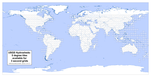
HydroSHEDS 5 degree index map (click for full size, 935K PNG)

Each tile in this map is labeled with the concatenated tile name representing the coordinates of the lower-left corner of each tile. For example, the tile for Rhode Island is “n40w075” with a lower left corner at 40°N latitude and 75°W longitude.

The fact that the tiles are measured in degrees means that this is an excellent case for using the plate carrée equirectangular projection, which has horizontal and vertical units of degrees. This is, of course, equivalent to what ArcMap shows when setting a data frame’s coordinate system to a “geographic” projection.

For convenience, you can also download the index in shapefile or GeoJSON format.
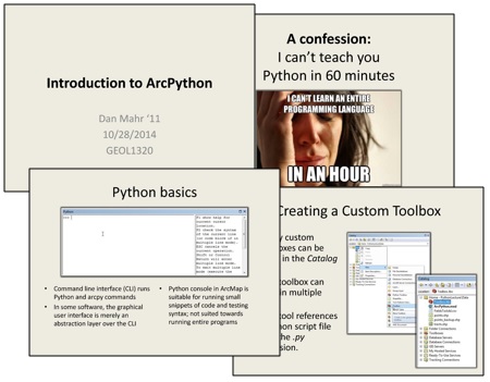
Introduction to ArcPython lecture

For the third year running, I returned to Brown to give a guest lecture about using Python in GIS for GEOL1320: Introduction to Geographic Information Systems for Environmental Applications. I’ve used ArcPython extensively in my work at Cadmus, and it’s exciting and heartening to be invited to lecture to GIS novices about the topic.

Nonetheless, the lecture is a challenge. I don’t have any formal experience teaching undergraduates. Moreover, it’s practically impossible to teach a programming language (even one as intuitive as Python) in an 80 minute time slot, let alone its nuanced GIS applications. Thus my strategy has been to think of the lecture as an icebreaker: a way to take away the barriers and scare-factor associated with getting started with Python. After a brief introduction, I showcased a few real-world examples of how I’ve used ArcPython in my work. Then the whole class worked through a live demo, doing a fairly simple task—adding fields to a feature class—using progressively more complex Python commands. Eventually, we even packed the final tool into a Python custom toolbox connected to a separate .py script file.

This year was definitely the most successful yet. The fact that students typed the commands themselves in a lab-format class made for a more engaging and effective class versus students watching me type in a lecture-format class. I hope these GIS novices got a good sense of what is possible with ArcPython. My slides are attached below.

Download slides (1.8MB .pptx)

Senior Thesis – Drivers of land-use change in Mato Grosso: A ten-year MODIS analysis

Senior thesis - PDF download (13.2MB)
Senior thesis – PDF download (13.2MB)

As part of my Bachelor of Science in Environmental Science degree program, I am required to write a senior thesis. After taking GEOL133 in Spring 2010, I knew I was interested in exploring additional topics in remote sensing. My GEOL133 professor, Jack Mustard, got me involved in some of his research examining agricultural extensification and intensification in the central Brazilian state of Mato Grosso. After two semesters of downloading data, learning IDL, processing tiles, testing smoothing techniques, and creating figures, this was the result.

I want to thank my advisors, Jack Mustard, Leah VanWey, and Chris Neill for their invaluable help, guidance, and feedback. Additional thanks to Lynn Carlson, Gillian Galford, Xi Yang, Rebecca de Sa, Shelby Riskin, Marcio Caparroz, Peter Klein, and Brett Lien for their help and assistance.

Abstract

The Brazilian state of Mato Grosso represents a hotspot of large-scale anthropogenic land-use change with major implications for the global carbon cycle, biodiversity, and regional climatic processes. Previous research has documented both the expansion of croplands into the state’s rainforest and cerrado biomes and the intensification of existing croplands through the increased prevalence of multi-cropping. Less closely examined are the socioeconomic drivers of this agricultural growth. In this study, we use the latest version of 250 meter vegetation indices satellite data from Terra-MODIS and a phenology classification algorithm to characterize cropland expansion and multi-cropping intensification in Mato Grosso on a yearly basis from August 2000 through August 2010. We compared these land-use changes to variations in commodity prices, exchange rates, export destinations, and other relevant events. We observed a 25,095 km2 increase in the total area of cropland, while the percentage of cropland classified as multi-cropped grew from 37.6% to 64.4%. These changes correlated most closely to the exchange rate of the Brazilian real to the currencies of its primary soybean export destinations (Europe and China). Significant appreciation of the real since 2009 would suggest decreased cropland expansion and multi-cropping intensification going forward. However, recent rises in commodity prices and sweeping changes proposed to Brazil’s Forest Code may encourage continued or increased land-use change in the near future.